Visualization

Set up

Load the needed packages.

suppressPackageStartupMessages({
library(dplyr)
library(sf)
library(ggplot2)
library(cmocean)
library(maxnet)
library(stars)
})

Set the file location.

here::i_am("tutorial/Steps_visualization.Rmd")

here() starts at /Users/eli.holmes/Documents/GitHub/ohw23_proj_marinesdms

Load the model

We saved this in the previous step. Has the sdm.model, occ.points, abs.points, and env.stars.crop.

fil <- here::here("data", "models", "io-turtle.RData")
load(fil)

Load region files. We created our region objects in a separate file Region data and saved these in data/region. We will load these now.

Load the bounding box polygon and create a bounding box.

#Loading bounding box for the area of interest
fil <- here::here("data", "region", "BoundingBox.shp")
extent_polygon <- sf::read_sf(fil)
bbox <- sf::st_bbox(extent_polygon)

Predicting

clamp <- TRUE       # see ?predict.maxnet for details
type <- "cloglog"
predicted <- predict(sdm.model, env.stars.crop, clamp = clamp, type = type)
predicted

stars object with 2 dimensions and 1 attribute
attribute(s):
           Min.   1st Qu.    Median      Mean   3rd Qu.      Max.  NA's
pred  0.0047245 0.1095251 0.1561052 0.1812027 0.2369365 0.9996747 52802
dimension(s):
  from   to offset    delta                       refsys x/y
x 2663 2942   -180  0.08333 +proj=longlat +datum=WGS8... [x]
y  695 1082     90 -0.08333 +proj=longlat +datum=WGS8... [y]

Visualization

ggplot() +
  geom_stars(data = predicted) +
  scale_fill_cmocean(name = "ice", direction = -1, guide = guide_colorbar(barwidth = 1, barheight = 10, ticks = FALSE, nbin = 1000, frame.colour = "black"), limits = c(0, 1)) +
  theme_linedraw() +
  coord_equal() +
  theme(panel.background = element_blank(),
        panel.grid.major = element_blank(),
        panel.grid.minor = element_blank()) +
  labs(title = "Loggerhead and green sea turtle SDM in the Arabian Sea",
       x = "Longitude",
       y = "Latitude",
       fill = "Probability",
       shape = "Species (presence)",
       subtitle = "Environmental predictors: mean SS temp, mean SS salinity, mean bathymetry, \nmean pH, mean DO, mean SS chlorophyll-a, mean SS nitrate") +
  geom_point(occ.points, mapping = aes(shape = common.name, geometry = geometry), stat = "sf_coordinates", alpha = 0.3, color = "purple") +
  #scale_x_continuous(breaks = seq(40, 70, 10), limits = c(42, 70))+
  scale_y_continuous(breaks = seq(0, 30, 10))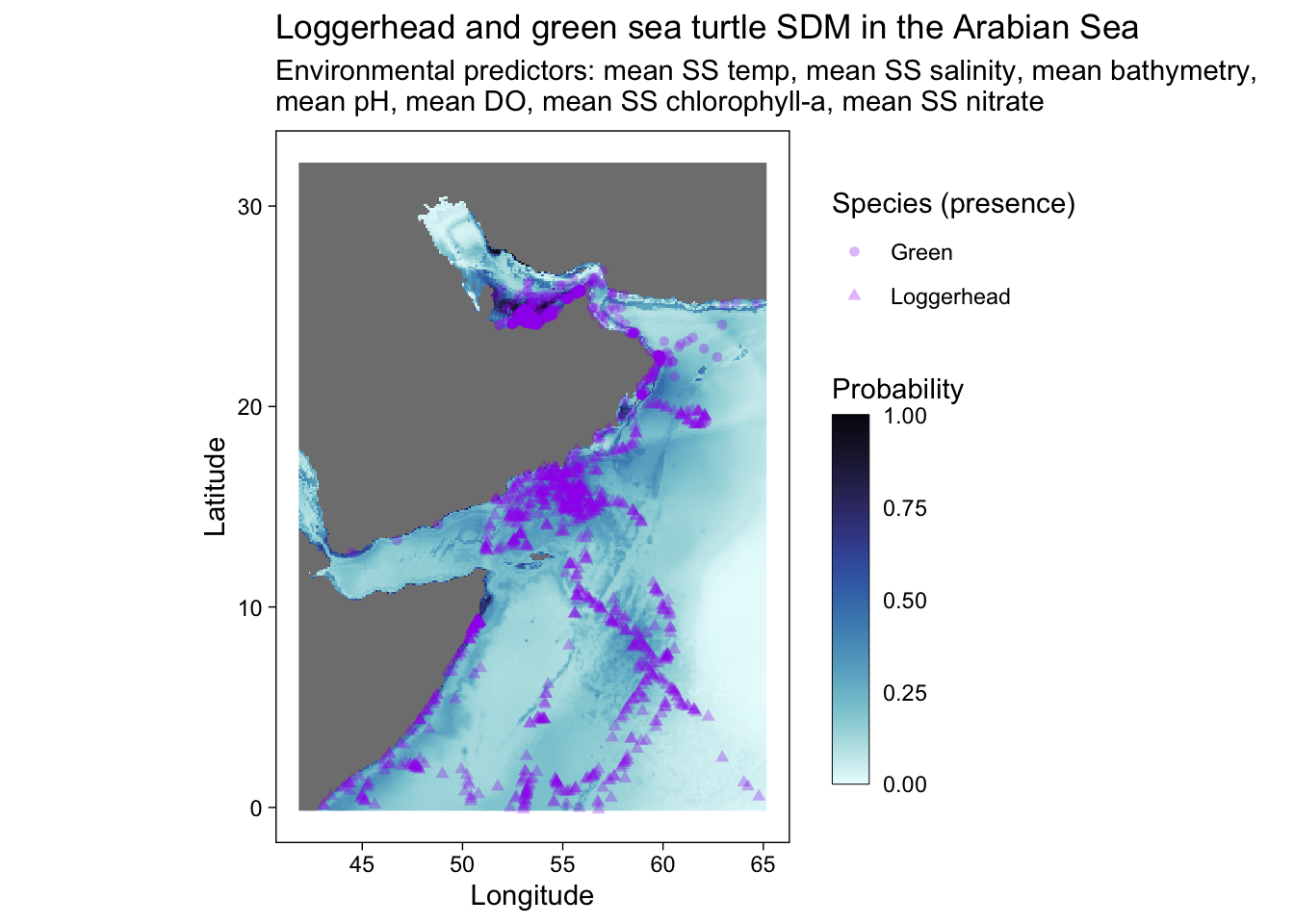

# ggsave("SDM_loggerhead_green_w points.pdf", height = 6, width = 8.5)

# ggplot - without occurrence data points

ggplot() +
  geom_stars(data = predicted) +
  scale_fill_cmocean(name = "ice", direction = -1, guide = guide_colorbar(barwidth = 1, barheight = 10, ticks = FALSE, nbin = 1000, frame.colour = "black"), limits = c(0, 1)) +
  theme_linedraw() +
  theme(panel.background = element_blank(),
        panel.grid.major = element_blank(),
        panel.grid.minor = element_blank()) +
  labs(title = "Loggerhead and green sea turtle SDM in the Arabian Sea",
       x = "Longitude",
       y = "Latitude",
       fill = "Probability",
       shape = "Species (presence)",
       subtitle = "Environmental predictors: mean SS temp, mean SS salinity, mean bathymetry,\nmean pH, mean DO, mean SS chlorophyll-a, mean SS nitrate") +
  #geom_point(occ.points, mapping = aes(shape = common.name, geometry = geometry), stat = "sf_coordinates", alpha = 0.3, color = "purple") +
  #scale_x_continuous(breaks = seq(40, 70, 10), limits = c(42, 70))+
  scale_y_continuous(breaks = seq(0, 30, 10))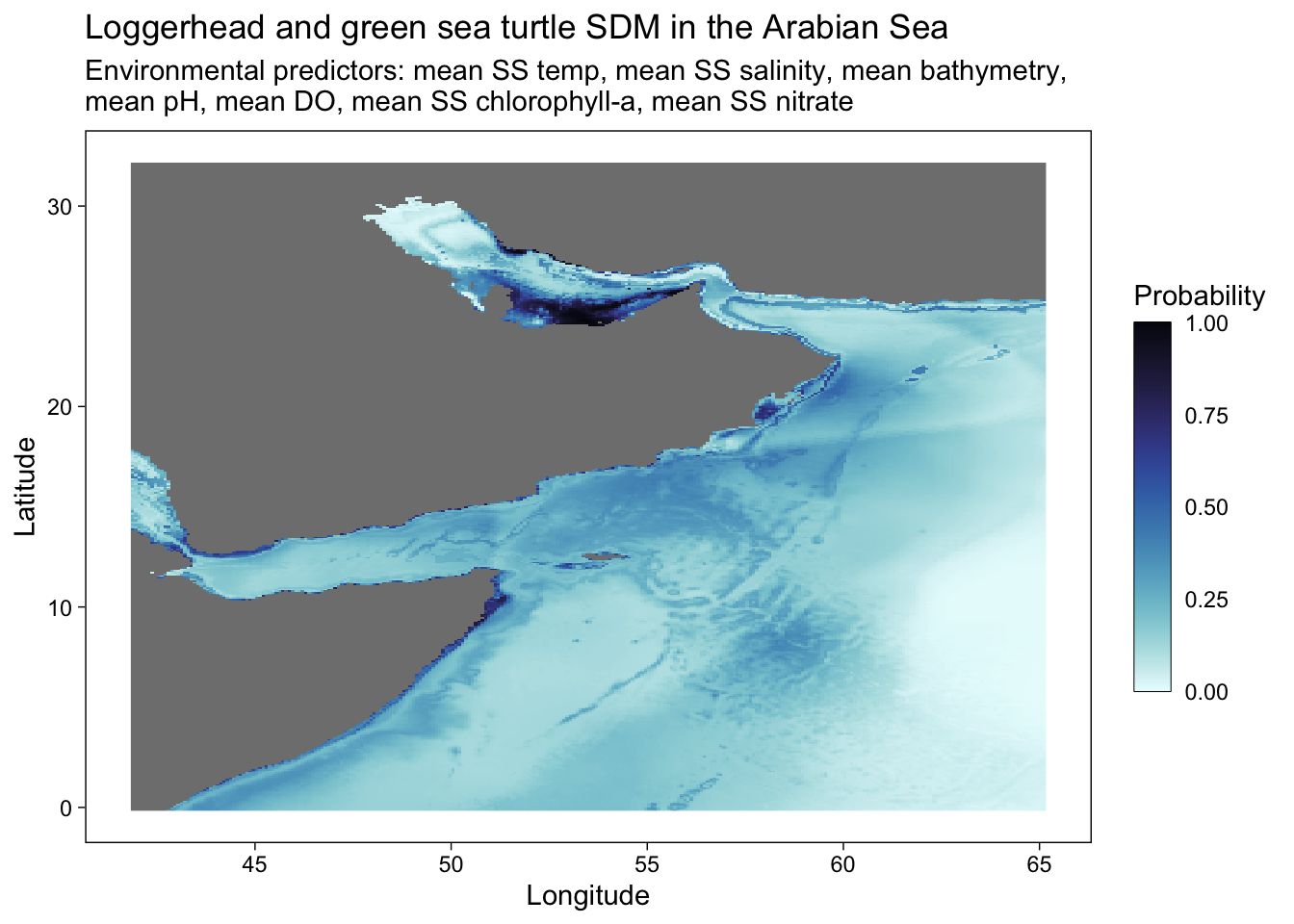

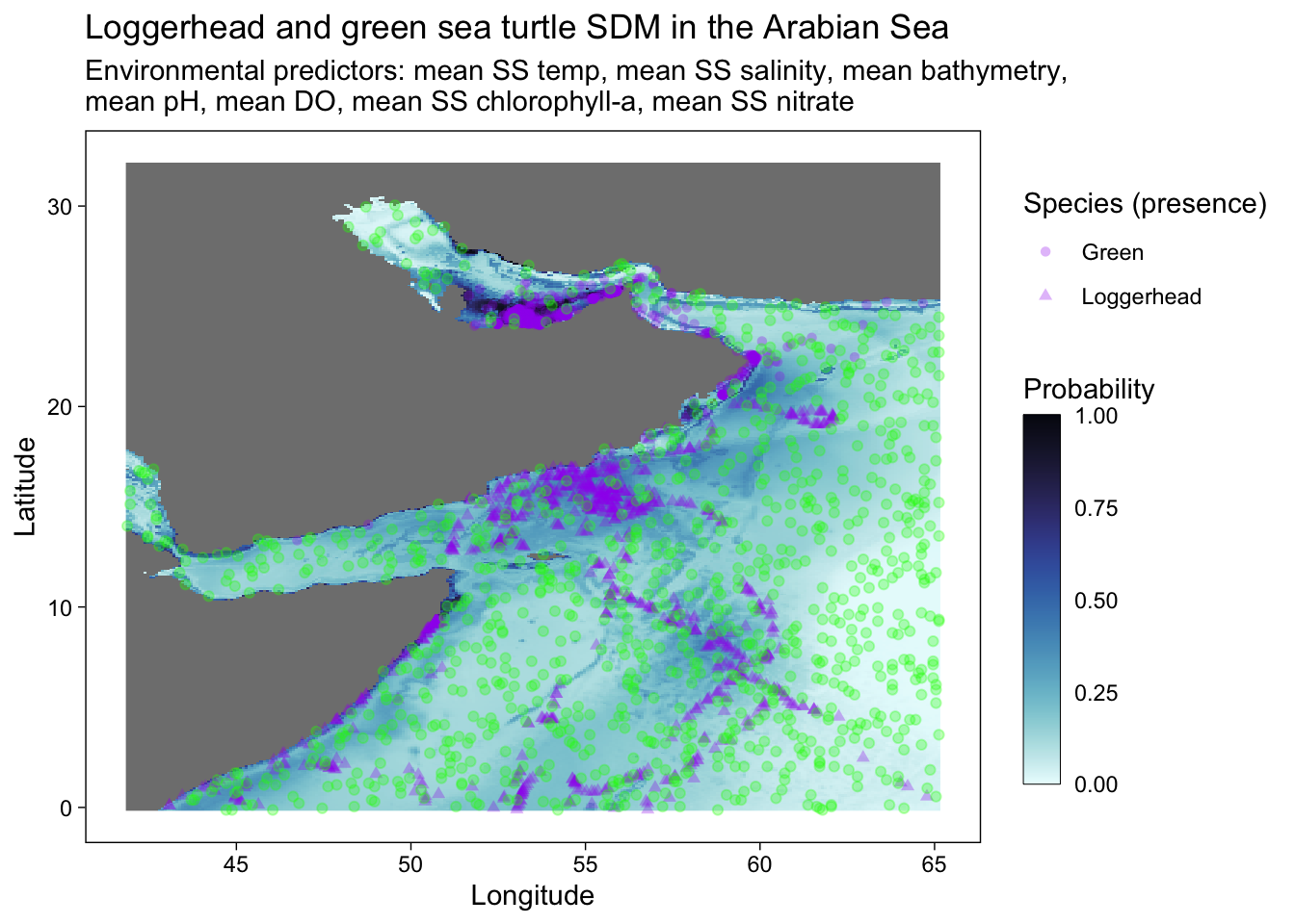
# ggsave("SDM_loggerhead_green.pdf", height = 6, width = 8.5)

# ggplot - with occurrence (purple) and absence (green) data points

ggplot() +
  geom_stars(data = predicted) +
  scale_fill_cmocean(name = "ice", direction = -1, guide = guide_colorbar(barwidth = 1, barheight = 10, ticks = FALSE, nbin = 1000, frame.colour = "black"), limits = c(0, 1)) +
  theme_linedraw() +
  theme(panel.background = element_blank(),
        panel.grid.major = element_blank(),
        panel.grid.minor = element_blank()) +
  labs(title = "Loggerhead and green sea turtle SDM in the Arabian Sea",
       x = "Longitude",
       y = "Latitude",
       fill = "Probability",
       shape = "Species (presence)",
       subtitle = "Environmental predictors: mean SS temp, mean SS salinity, mean bathymetry, \nmean pH, mean DO, mean SS chlorophyll-a, mean SS nitrate") +
  geom_point(occ.points, mapping = aes(shape = common.name, geometry = geometry), stat = "sf_coordinates", alpha = 0.3, color = "purple") +
  #scale_x_continuous(breaks = seq(40, 70, 10), limits = c(42, 70))+
  scale_y_continuous(breaks = seq(0, 30, 10)) +
  geom_point(abs.points, mapping = aes(geometry = geometry), stat = "sf_coordinates", alpha = 0.3, color = "green") # adding in absence data