Getting background data from OBIS

In this notebook, we will explore three approaches to create background samples, aka pseudo absences. These are points where turtles were not recorded. These absences are needed for our choice of species distribution model algorithm. “Absences” does not mean that turtle could not be sighted here but that we have no records at these locations, either because we didn’t look or looked and didn’t see them.

These three approaches are as follows:

Get occurrences for marine species from OBIS using the robis package, and use their locations as the locations for absences.
Select random locations using gridded environmental data as a base for our sampling.
Select random locations using a polygon drawn around our presence locations.

In both cases, points will be constrained to fit within our area of interest.

Loading libraries

#Deal with spatial data
library(sf)
#Base maps and plotting spatial data
library(rnaturalearth)
library(mapview)
library(raster)
#Data visualisation and manipulation
library(tidyverse)
#Find files easily
library(here)
#Access to OBIS
library(robis)
#SDM
library(sdmpredictors)
library(dismo)
library(ggspatial)

Set-up

Setting base directories

These directories contain the biological data (i.e., presence locations of loggerhead sea turtles) and environmental data.

#Setting directories containing input data
dir_data <- file.path(here::here(), "data/raw-bio")
dir_env <- file.path(here::here(), "data/env")

Loading bounding box for region of interest

In the Region page, we created a bounding box for our region of interest. We will load this bounding box here to spatially constrain our data.

#Loading bounding box for the area of interest
fil <- here::here("data", "region", "BoundingBox.shp")
extent_polygon <- read_sf(fil)

#Extract polygon geometry 
pol_geometry <- st_as_text(extent_polygon$geometry)

Approach 1: Use other species

In this approach we use other marine species presence locations as our locations for our background samples.

Getting occurrence data from OBIS

We will use robis to get observations for marine species from OBIS within our bounding box. OBIS data includes about 100 different columns, but not all of these columns are relevant to us. We will define the columns that we need and then we will perform a search of the OBIS database.

Defining relevant columns

cols.to.use <- c("scientificName", "dateIdentified", "eventDate", "decimalLatitude", "decimalLongitude", "coordinateUncertaintyInMeters", "bathymetry",  "shoredistance", "sst", "sss")

Querying OBIS

By setting the wrims parameter to TRUE we include observations of species registerd in the World Register of Introduced Marine Species (WRiMS).

#Applying bounding box and including WRiMS species
background <- occurrence(geometry = pol_geometry, wrims = TRUE, 
                         #DNA data is not needed, subsetting columns of interest
                         dna = FALSE, fields = cols.to.use,
                         #Excluding records labelled as being on land
                         exclude = "ON_LAND")


Retrieved 5000 records of approximately 20511 (24%)
Retrieved 10000 records of
approximately 20511 (48%)
Retrieved 15000 records of approximately 20511
(73%)
Retrieved 20000 records of approximately 20511 (97%)
Retrieved 20511
records of approximately 20511 (100%)

Saving background data

#Setting full file path to save background information
file_path_out <- file.path(dir_data, "io-background.csv")

#Saving background data as csv
write_csv(background, file_path_out)

(Optional) Load background data

If you have previously downloaded the background data, you can simply load the data to the environment instead of downloading it again. To do this, you can use the code below.

#Find background file in our biological data folder
file_path_bg <- list.files(dir_data, pattern = "background", full.names = TRUE)

#Load file
background_1 <- read_csv(file_path_bg)

Plotting background data

We will create a map with all the observations we obtained from OBIS within our region of interest.

First we will load the region map that was saved in the Region page

fil <- here::here("data", "region", "region_map_label.rda")
load(fil)

Saving map into variable

# load our base map and add points
region_map_label +
  geom_point(data = background, 
             #Point to coordinates for background points
             aes(x = decimalLongitude, y = decimalLatitude), 
             #Changing color and size of points for background data
             color = "red", size = 0.1)

Scale on map varies by more than 10%, scale bar may be inaccurate

Warning: Removed 231 rows containing missing values (`geom_text()`).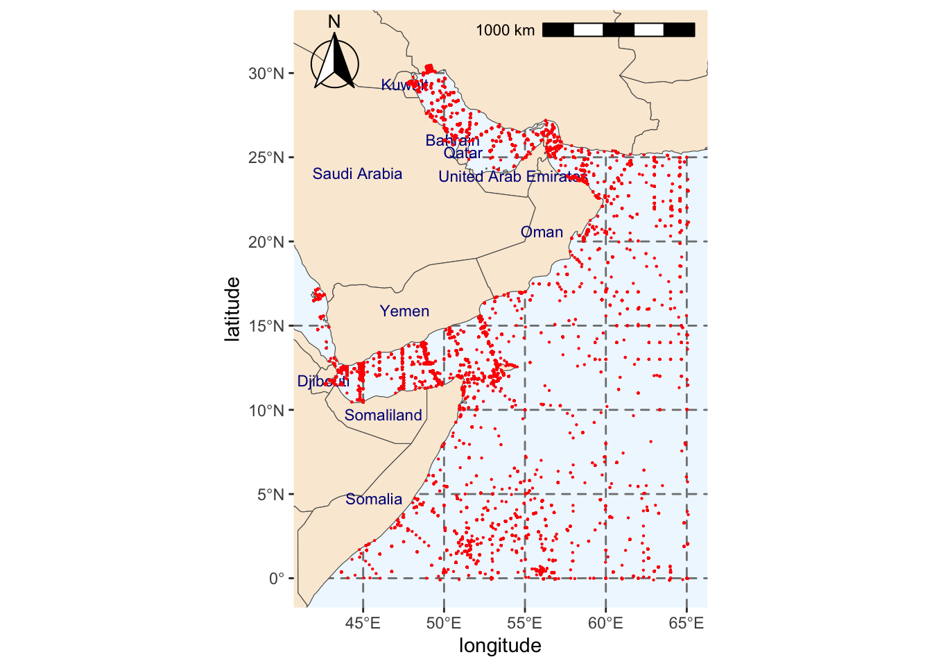

As you can see from the map above, this approach is not truly random. This is why we are including a second method to create background samples.

Approach 2. Random points in our region

This section has been adapted from this online tutorial.

Loading raster layer for area of interest

We will be using sdmpredictors for our environmental data layers (variables). We need to load a raster layer from sdmpredictors so we can sample locations from this raster. It doesn’t matter what variable we use, it just needs to not have NAs. Using a marine layer from sdmpredictors ensures that we will not sample from the land. See the sdmpredictors section for discussion of accessing rasters with sdmpredictors and how to find out what layers are available.

We used a bathymetery layer: “MS_bathy_5m”. We will load this data and crop it using our bounding box.

#Set default directory for environmental data
options(sdmpredictors_datadir = dir_env)
#Loading bathymetry
env_stack <- load_layers("MS_bathy_5m") %>% 
  #Cropping to our area of interest
  crop(extent_polygon)

We can plot the cropped bathymetry to ensure it matches our study region and we did not make any mistakes.

plot(env_stack)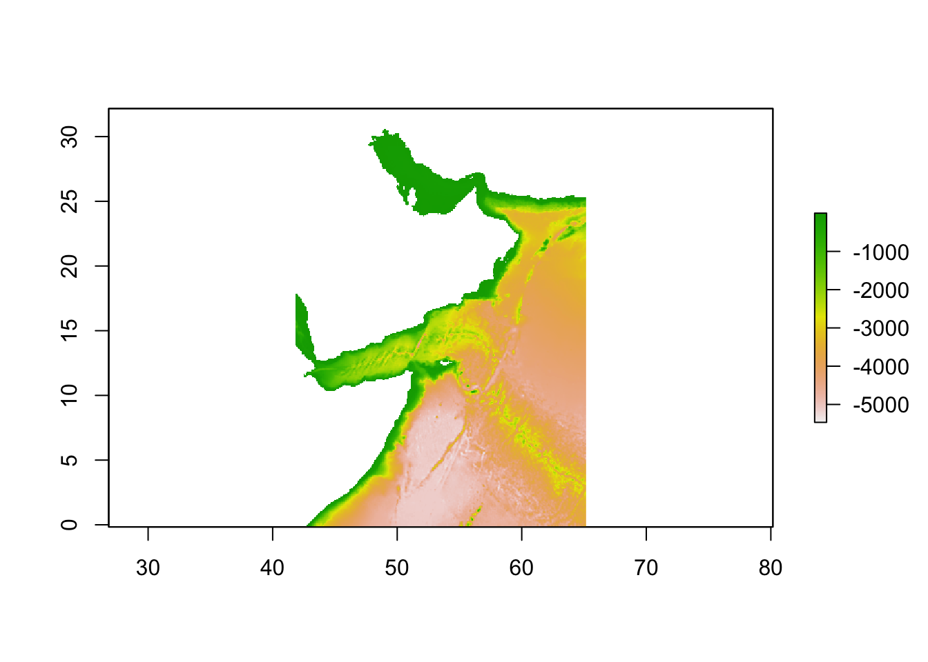

We can see the outline of our area of interest. Now we can continue with creating our background points.

Sample points from bathymetry layer

Using the dismo package, we will create random points over the bathymetry layer that we will use as background points. In this example, we have chosen to produce 1000 background points.

It is worth noting that the distribution and number of background points has a strong influence on SDM results. See the README file for resources discussing this issue.

#Setting seed for reproducibility
set.seed(42)

#Setting number of background points required
nsamp <- 1000

#Create background points
background <- randomPoints(env_stack, nsamp) %>% 
  #Transform to tibble
  as_tibble() %>% 
  #Transform to sf object
  st_as_sf(coords = c("x", "y"), crs = 4326)

Plotting results

We will plot results to make sure our background points are in the ocean only. Here we use an alternate why to plot points on a map.

mapview(background, col.regions = "gray")

Warning in cbind(`Feature ID` = fid, mat): number of rows of result is not a
multiple of vector length (arg 1)

Saving background samples

We can now save the background locations to our local machine.

absence_geo <- file.path(dir_data, "absence.geojson")
pts_absence_csv <- file.path(dir_data, "pts_absence.csv")
st_write(background, pts_absence_csv, layer_options = "GEOMETRY=AS_XY", append = FALSE)

Deleting layer `pts_absence' using driver `CSV'
Writing layer `pts_absence' to data source 
  `/Users/eli.holmes/Documents/GitHub/ohw23_proj_marinesdms/data/raw-bio/pts_absence.csv' using driver `CSV'
options:        GEOMETRY=AS_XY 
Updating existing layer pts_absence
Writing 1000 features with 0 fields and geometry type Point.

Approach 3. Random points a convex hull

This section has been adapted from this online tutorial and this online tutorial.

The next notebook will discuss how to get environmental data that we will use as inputs in our SDM from the sdmpredictors package.