Get background data

We used the random samples within our region of interest to generate a file with the locations for our absences.

Set up

library(ggplot2)
library(sf)

Linking to GEOS 3.11.0, GDAL 3.5.3, PROJ 9.1.0; sf_use_s2() is TRUE

library("rnaturalearth")
library("rnaturalearthdata")

Attaching package: 'rnaturalearthdata'

The following object is masked from 'package:rnaturalearth':

    countries110

library(raster)

Loading required package: sp

library(tidyverse)

── Attaching core tidyverse packages ──────────────────────── tidyverse 2.0.0 ──
✔ dplyr     1.1.3     ✔ readr     2.1.4
✔ forcats   1.0.0     ✔ stringr   1.5.0
✔ lubridate 1.9.2     ✔ tibble    3.2.1
✔ purrr     1.0.1     ✔ tidyr     1.3.0

── Conflicts ────────────────────────────────────────── tidyverse_conflicts() ──
✖ tidyr::extract() masks raster::extract()
✖ dplyr::filter()  masks stats::filter()
✖ dplyr::lag()     masks stats::lag()
✖ dplyr::select()  masks raster::select()
ℹ Use the conflicted package (<http://conflicted.r-lib.org/>) to force all conflicts to become errors

dir_data <- file.path(here::here(), "data", "raw-bio")
dir_env <- file.path(here::here(), "data", "env")
redo <- TRUE

Load region info

Load the bounding box polygon and create a bounding box.

#Loading bounding box for the area of interest
fil <- here::here("data", "region", "BoundingBox.shp")
extent_polygon <- sf::read_sf(fil)
bbox <- sf::st_bbox(extent_polygon)
wkt_geometry <- extent_polygon$geometry %>% st_as_text()

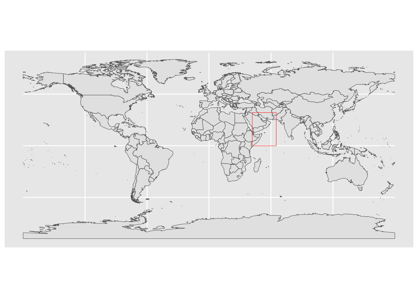
Make a map of our region so we know we have the right area.

world <- ne_countries(scale = "medium", returnclass = "sf")
ggplot(data = world) + geom_sf() +
  geom_sf(data = extent_polygon, color = "red", fill=NA)

Random samples

This is adapted from here.

Get a marine raster layer

We just need one because we use this to sample lat/lons from the marine environment.

# set a default data directory
options(sdmpredictors_datadir = dir_env)

# choosing marine
env_datasets <- sdmpredictors::list_datasets(terrestrial = FALSE, marine = TRUE)
env_layers <- sdmpredictors::list_layers("MARSPEC")
env_stack <- sdmpredictors::load_layers("MS_bathy_5m")
env_stack <- env_stack %>% raster::crop(extent_polygon)

Plot to check that the layer looks ok. This is bathymetry.

plot(env_stack)

Next we sample points from this

It returns a sf points object.

nsamp <- 1000
absence <- dismo::randomPoints(env_stack[[1]], nsamp) %>% 
    as_tibble() %>% 
    st_as_sf(coords = c("x", "y"), crs = 4326)

mapview::mapview(absence, col.regions = "gray")

Warning in cbind(`Feature ID` = fid, mat): number of rows of result is not a
multiple of vector length (arg 1)

Save

Save the absence locations to a file.

absence_geo <- file.path(dir_data, "absence.geojson")
pts_absence_csv <- file.path(dir_data, "pts_absence.csv")
st_write(absence, pts_absence_csv, layer_options = "GEOMETRY=AS_XY", append=FALSE)

Deleting layer `pts_absence' using driver `CSV'
Writing layer `pts_absence' to data source 
  `/Users/eli.holmes/Documents/GitHub/ohw23_proj_marinesdms/data/raw-bio/pts_absence.csv' using driver `CSV'
options:        GEOMETRY=AS_XY 
Updating existing layer pts_absence
Writing 1000 features with 0 fields and geometry type Point.