Setting up the region

As a preliminary, we will define some shape files and plots of our region that we will use in later steps.

Load libraries

#Dealing with spatial data
library(sf)
#Getting base maps
library(rnaturalearth)
#Data manipulation and visualisation
library(tidyverse)
library(janitor)
library(ggspatial)

Create a bounding box

We will use a bounding box for the region of our interest (Arabian Sea and the Bay of Bengal) to extract C. caretta data relevant to our study area.

#We create a bounding box using minimum and maximum coordinate pairs
extent_polygon <- st_bbox(c(xmin = 41.875, xmax = 65.125, 
                            ymax = -0.125, ymin = 32.125), 
                          #Assign reference system
                          crs = st_crs(4326)) %>% 
  #Turn into sf object
  st_as_sfc()

#Extract polygon geometry 
pol_geometry <- st_as_text(extent_polygon[[1]])

#Saving bounding box for future use
fil <- here::here("data", "region", "BoundingBox.shp")
write_sf(extent_polygon, fil)

Create a world map

We can create a world map to show where our study region is. ### Plotting region of interest This allows us to check our polygon of interest is located in the correct region.

#Getting base map
world <- ne_countries(scale = "medium", returnclass = "sf")

#Plotting map
world_box <- ggplot() + 
  #Adding base map
  geom_sf(data = world) +
  #Adding bounding box
  geom_sf(data = extent_polygon, color = "red", fill = NA)+
  #Setting theme of plots to not include a grey background
  theme_bw()
fil <- here::here("data", "region", "world_box.rda")
save(world_box, file=fil)

world_box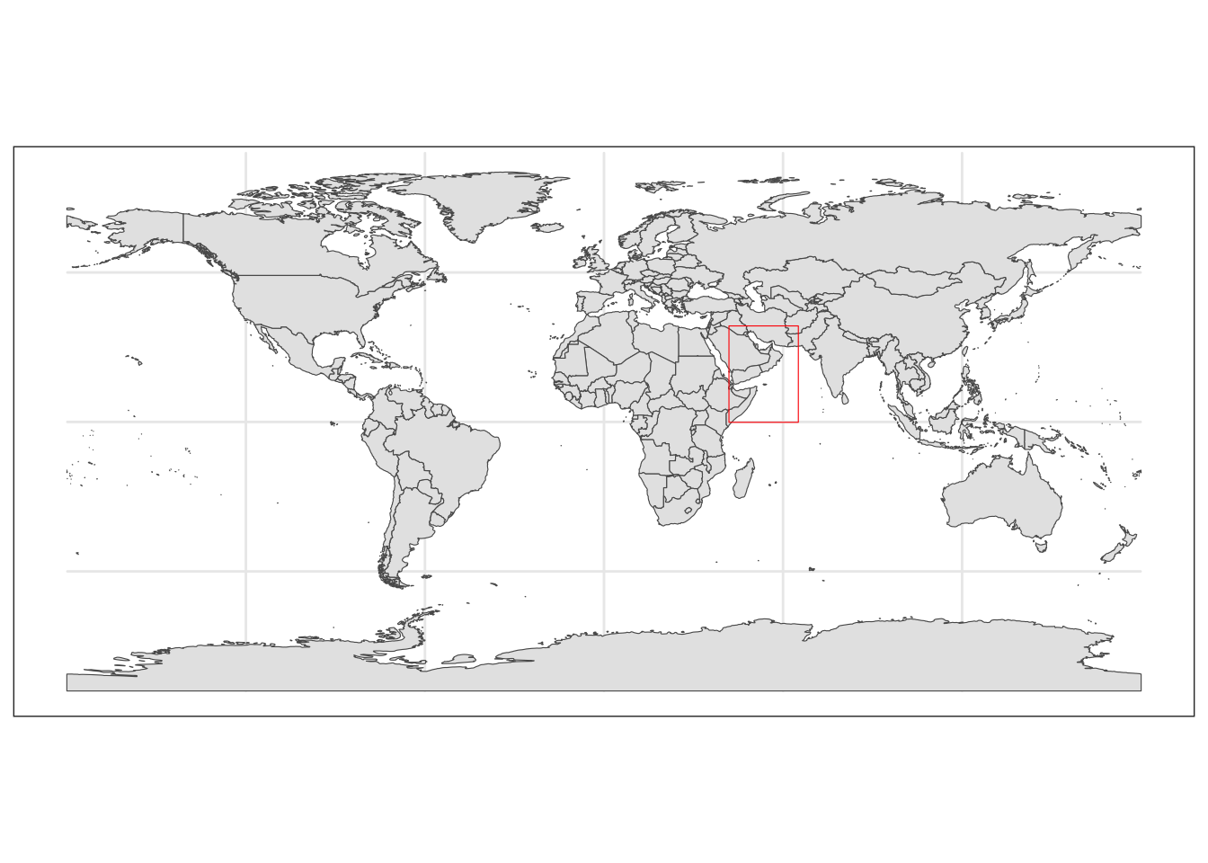

Create a region map

First we create a base map of our region and save it.

base_region_map <- ggplot()+
  #Adding base layer (world map)
  geom_sf(data = world, fill = "antiquewhite")+
  #Constraining map to original bounding box
  lims(x = c(st_bbox(extent_polygon)$xmin, st_bbox(extent_polygon)$xmax),
       y = c(st_bbox(extent_polygon)$ymin, st_bbox(extent_polygon)$ymax))
fil <- here::here("data", "region", "base_region_map.rda")
save(base_region_map, file=fil)

base_region_map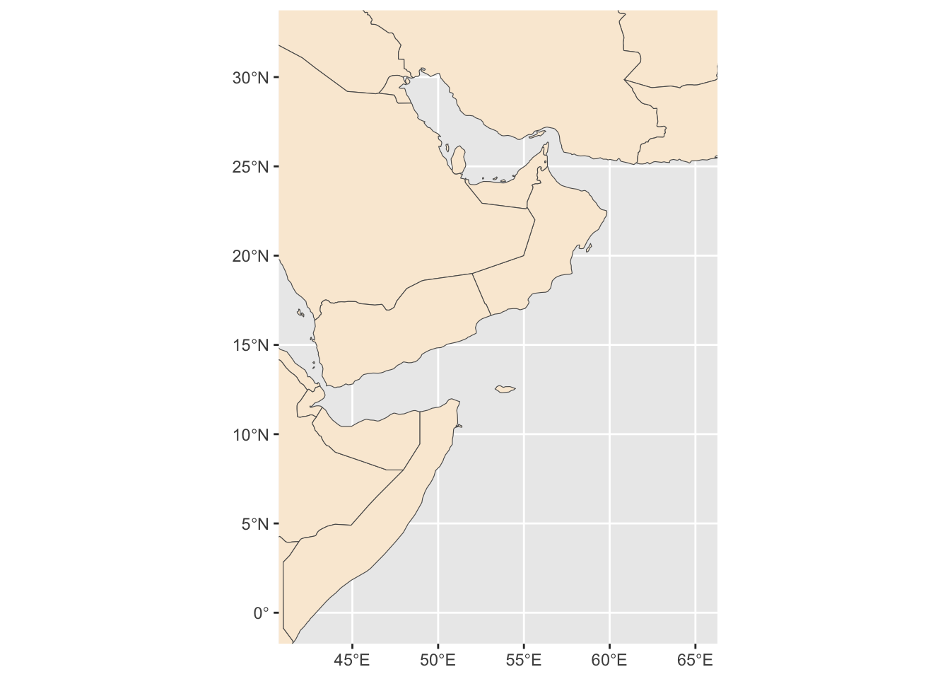

We will add some more features to our map: colors, scale and compass.

region_map <- base_region_map +
  #Add scale bar on the top right of the plot
  annotation_scale(location = "tr", width_hint = 0.5)+
  #Add north arrow on the top left of plot
  annotation_north_arrow(location = "tl", which_north = "true",
                         #Include small buffer from plot edge
                         pad_x = unit(0.01, "in"), pad_y = unit(0.05, "in"),
                         #Set style of north arrow
                         style = north_arrow_fancy_orienteering) +
  #Changing color, type and size of grid lines
  theme(panel.grid.major = element_line(color = gray(.5), linetype = "dashed", size = 0.5), 
  #Change background of map
  panel.background = element_rect(fill = "aliceblue")) +
  labs(x = "longitude", y = "latitude")

Warning: The `size` argument of `element_line()` is deprecated as of ggplot2 3.4.0.
ℹ Please use the `linewidth` argument instead.

fil <- here::here("data", "region", "region_map.rda")
save(region_map, file=fil)

region_map

Scale on map varies by more than 10%, scale bar may be inaccurate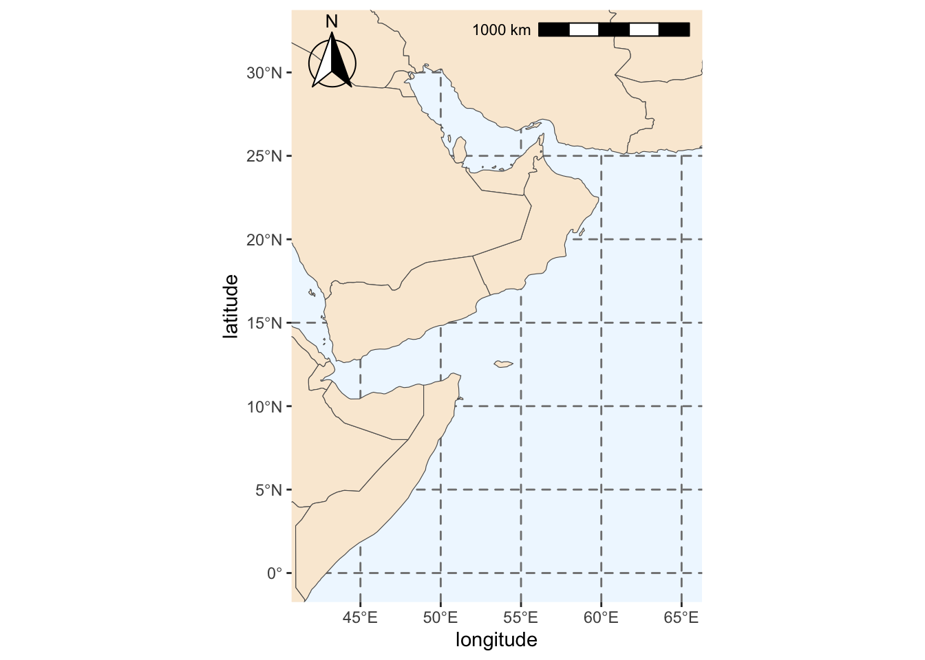

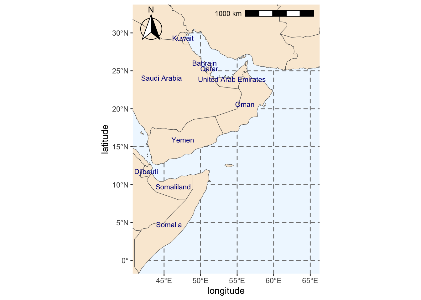
We add some labels for the countries.

#Extracting labels for countries in base map
world_points <- world %>% 
  st_make_valid(world) %>%
  #Getting centroids for all polygons in the world base map
  st_centroid(geometry) %>% 
  #Getting coordinates for each centroid
  st_coordinates() %>% 
  #Adding centroids to original base map
  bind_cols(world)

#Do not use spherical geometry
sf_use_s2(FALSE)

#Adding labels to map
region_map_label <- region_map +
  geom_text(data = world_points, 
            #Point to coordinates and column with country names
            aes(x = X, y = Y, label = name),
            #Changing color and size of labels
            color = "darkblue", size = 3, 
            #Avoid label overlap
            check_overlap = TRUE)
fil <- here::here("data", "region", "region_map_label.rda")
save(region_map_label, file=fil)

#Checking final map
region_map_label