Get turtle data

Here we download from OBIS using the robis package.

Set up

library(ggplot2)
library(sf)

Linking to GEOS 3.11.0, GDAL 3.5.3, PROJ 9.1.0; sf_use_s2() is TRUE

library("rnaturalearth")
library("rnaturalearthdata")

Attaching package: 'rnaturalearthdata'

The following object is masked from 'package:rnaturalearth':

    countries110

library(raster)

Loading required package: sp

library(tidyverse)

── Attaching core tidyverse packages ──────────────────────── tidyverse 2.0.0 ──
✔ dplyr     1.1.3     ✔ readr     2.1.4
✔ forcats   1.0.0     ✔ stringr   1.5.0
✔ lubridate 1.9.2     ✔ tibble    3.2.1
✔ purrr     1.0.1     ✔ tidyr     1.3.0

── Conflicts ────────────────────────────────────────── tidyverse_conflicts() ──
✖ tidyr::extract() masks raster::extract()
✖ dplyr::filter()  masks stats::filter()
✖ dplyr::lag()     masks stats::lag()
✖ dplyr::select()  masks raster::select()
ℹ Use the conflicted package (<http://conflicted.r-lib.org/>) to force all conflicts to become errors

library(robis)

Attaching package: 'robis'

The following object is masked from 'package:raster':

    area

Load the region info

Load the bounding box polygon and create a bounding box.

#Loading bounding box for the area of interest
fil <- here::here("data", "region", "BoundingBox.shp")
extent_polygon <- sf::read_sf(fil)
bbox <- sf::st_bbox(extent_polygon)
wkt_geometry <- extent_polygon$geometry %>% st_as_text()

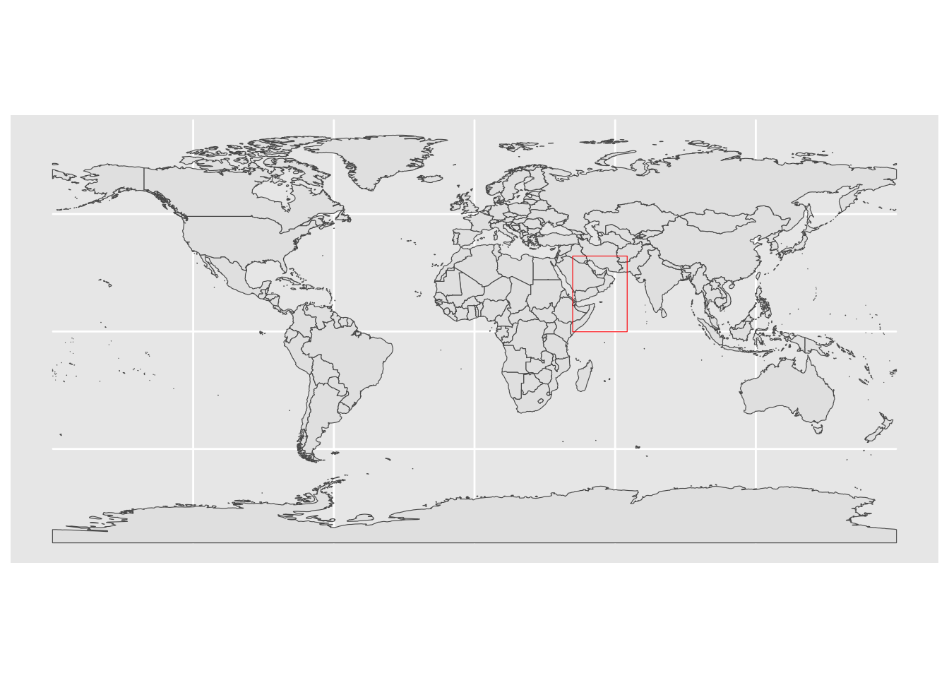
Make a map of our region so we know we have the right area.

world <- ne_countries(scale = "medium", returnclass = "sf")
ggplot(data = world) + geom_sf() +
  geom_sf(data = extent_polygon, color = "red", fill=NA)

Get occurrence data from robis

We will download data for four sea turtles found in the Arabian sea and save to one file. We will use the occurrence() function in the robis package.

spp <- c("Chelonia mydas", "Caretta caretta", "Eretmochelys imbricata", "Lepidochelys olivacea", "Natator depressus", "Dermochelys coriacea")

obs <- robis::occurrence(spp, startdate = as.Date("2000-01-01"), geometry = wkt_geometry)

This has many columns that we don’t need. We reduced to fewer columns.

cols.to.use <- c("occurrenceID", "scientificName", 
                 "dateIdentified", "eventDate", 
                 "decimalLatitude", "decimalLongitude", "coordinateUncertaintyInMeters",
                 "individualCount","lifeStage", "sex",
                 "bathymetry",  "shoredistance", "sst", "sss")
obs <- obs[,cols.to.use]

We also added a cleaner date with YYYY-MM-DD format.

obs$date <- as.Date(obs$eventDate)

Save our data

Set up the file names

dir_data <- here::here("data", "raw-bio")
filname <- "io-sea-turtles"
obs_csv <- file.path(dir_data, paste0(filname, ".csv"))
obs_geo <- file.path(dir_data, paste0(filname, ".geojson"))
obs_gpkg <- file.path(dir_data, paste0(filname, ".gpkg"))

Change the data frame to a sf dataframe.

obs_sf <- obs %>% 
    sf::st_as_sf(
      coords = c("decimalLongitude", "decimalLatitude"),
      crs = st_crs(4326))

Save files in different formats to facilitate loading into geospatial packages.

redo   <- TRUE

if (!file.exists(obs_csv) | redo)  readr::write_csv(obs, obs_csv)
if (!file.exists(obs_geo) | redo)  sf::write_sf(obs_sf, obs_geo, delete_dsn=TRUE)
if (!file.exists(obs_gpkg) | redo)  sf::write_sf(obs_sf, obs_gpkg, delete_dsn=TRUE)

Later we can reload our data as

tmp <- sf::read_sf(obs_gpkg)
class(tmp)

Clean and prep data

Here we clean and prepare the data for our model and save to a new file name.

Load data in

# presence data
fil <- here::here("data", "raw-bio", "io-sea-turtles.csv")
io.turtles <- read.csv(fil)

Clean the data

Select species.

# turtle species we're interested in
spp <- c("Chelonia mydas", "Caretta caretta", "Eretmochelys imbricata", "Lepidochelys olivacea", "Natator depressus", "Dermochelys coriacea") 

# subsetting all the occurence data to just those turtles 
occ <- io.turtles %>% 
  subset(scientificName == spp) 

# subset the occurences to include just those in the water
occ <- occ %>% 
  subset(bathymetry > 0 & shoredistance > 0 & coordinateUncertaintyInMeters < 200)

# seeing how often each species occurs
table(occ$scientificName) 

Caretta caretta  Chelonia mydas 
            874            1190 

After cleaning we discover that we only have loggerhead and green sea turtles.

Select the needed columns

Select columns and add a common name column.

colnames(occ)

 [1] "occurrenceID"                  "scientificName"               
 [3] "dateIdentified"                "eventDate"                    
 [5] "decimalLatitude"               "decimalLongitude"             
 [7] "coordinateUncertaintyInMeters" "individualCount"              
 [9] "lifeStage"                     "sex"                          
[11] "bathymetry"                    "shoredistance"                
[13] "sst"                           "sss"                          
[15] "date"                         

We want these. The last two are sea surface temperature and salinity.

cols <- c("scientificName", "eventDate", "decimalLatitude", "decimalLongitude", "lifeStage", "bathymetry", "sst", "sss")

Subset the columns.

occ.sub <- occ %>% dplyr::select(all_of(cols))

Fix the event date to a date format.

occ.sub$eventDate <- lubridate::ymd_hms(occ.sub$eventDate) 

Change the column names.

colnames(occ.sub) <- c("sci.name", "obsv.datetime", "lat", "lon", "life.stage", "bathy", "SST", "SSS")

Add common.name column.

occ.sub <- occ.sub %>% 
  mutate(common.name = case_when(sci.name == "Caretta caretta" ~ "Loggerhead",
                                 sci.name == "Chelonia mydas" ~ "Green"))

Save the cleaned file

Save our data

Set up the file names

dir_data <- here::here("data", "raw-bio")
fil <- "io-sea-turtles-clean.csv"
obs_csv <- here::here(dir_data, fil)
if (!file.exists(obs_csv))  readr::write_csv(occ.sub, obs_csv)