Saving region files

As a preliminary, we will define some shape files and plots of our region that we will use in later steps.

Load libraries

library(sf)
library(rnaturalearth)
library(tidyverse)
library(janitor)
library(ggspatial)

Create a bounding box

Our interest is the Persian Gulf and northern Arabian Sea.

We create a bounding box using minimum and maximum coordinate pairs and assign a standared WGS 84 coordinate reference system. We will turn this into a polygon and then an sf object.

bbox <- sf::st_bbox(c(xmin = 41.875, xmax = 65.125, ymax = -0.125, ymin = 32.125), 
                          crs = sf::st_crs(4326))
# this creates a sf object with a sfs_POLYGON from which we can get a polygon string
extent_polygon <-  bbox %>% sf::st_as_sfc() %>% st_sf()

Save

Saving the bounding box for future use.

fil <- here::here("data", "region", "BoundingBox.shp")
write_sf(extent_polygon, fil)

We will also save the polygon in string format. The polygon text is the first element in the object.

pol_geometry <-  extent_polygon$geometry %>% sf::st_as_text()
fil <- here::here("data", "region", "pol_geometry.txt")
writeLines(pol_geometry, fil)

Create a world map

We can create a world map to show where our study region is and save these for later use.

Plotting region of interest

This allows us to check our polygon of interest is located in the correct region.

#Getting base map
world <- ne_countries(scale = "medium", returnclass = "sf")

#Plotting map
world_box <- ggplot() + 
  #Adding base map
  geom_sf(data = world) +
  #Adding bounding box
  geom_sf(data = extent_polygon, color = "red", fill = NA)+
  #Setting theme of plots to not include a grey background
  theme_bw()

world_box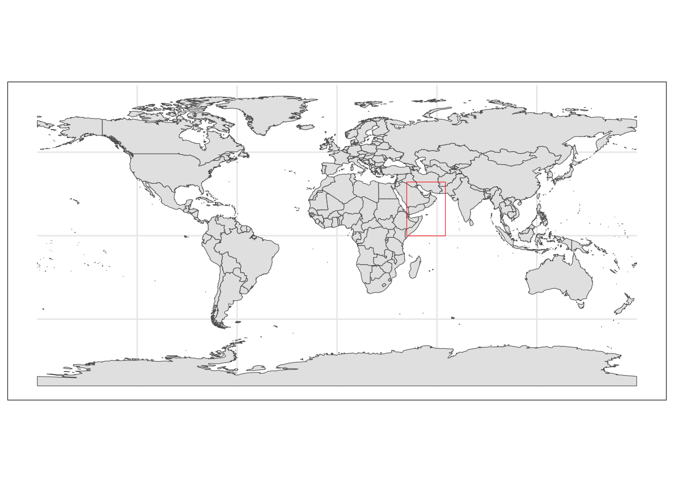

Save the plot.

fil <- here::here("data", "region", "world_box.rda")
save(world_box, file=fil)

Create a region map

We can create a base map of our region and save it.

base_region_map <- ggplot()+
  #Adding base layer (world map)
  geom_sf(data = world, fill = "antiquewhite")+
  #Constraining map to original bounding box
  lims(x = c(st_bbox(extent_polygon)$xmin, st_bbox(extent_polygon)$xmax),
       y = c(st_bbox(extent_polygon)$ymin, st_bbox(extent_polygon)$ymax))
base_region_map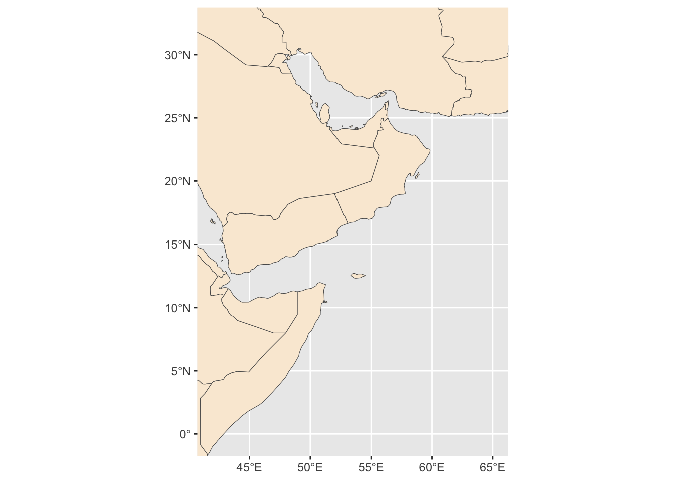

Save it

fil <- here::here("data", "region", "base_region_map.rda")
save(base_region_map, file=fil)

We will add some more features to our map: colors, scale and compass.

region_map <- base_region_map +
  #Add scale bar on the top right of the plot
  annotation_scale(location = "tr", width_hint = 0.5)+
  #Add north arrow on the top left of plot
  annotation_north_arrow(location = "tl", which_north = "true",
                         #Include small buffer from plot edge
                         pad_x = unit(0.01, "in"), pad_y = unit(0.05, "in"),
                         #Set style of north arrow
                         style = north_arrow_fancy_orienteering) +
  #Changing color, type and size of grid lines
  theme(panel.grid.major = element_line(color = gray(.5), linetype = "dashed", size = 0.5), 
  #Change background of map
  panel.background = element_rect(fill = "aliceblue")) +
  labs(x = "longitude", y = "latitude")

Warning: The `size` argument of `element_line()` is deprecated as of ggplot2 3.4.0.
ℹ Please use the `linewidth` argument instead.

region_map

Scale on map varies by more than 10%, scale bar may be inaccurate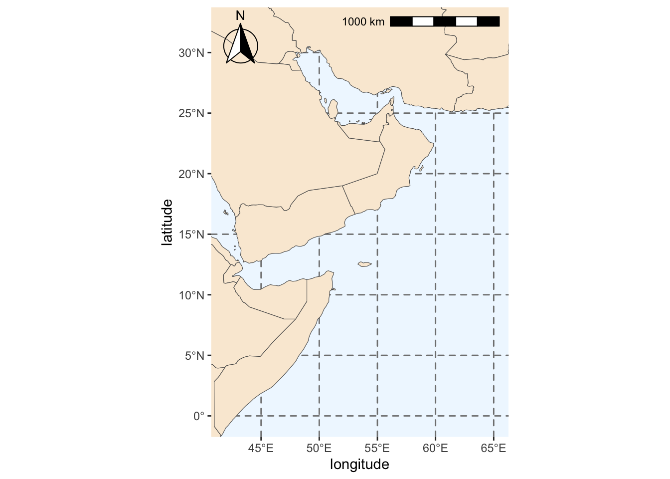

Save.

fil <- here::here("data", "region", "region_map.rda")
save(region_map, file=fil)

We add some labels for the countries.

#Extracting labels for countries in base map
world_points <- world %>% 
  st_make_valid(world) %>%
  #Getting centroids for all polygons in the world base map
  st_centroid(geometry) %>% 
  #Getting coordinates for each centroid
  st_coordinates() %>% 
  #Adding centroids to original base map
  bind_cols(world)

#Do not use spherical geometry
sf_use_s2(FALSE)

#Adding labels to map
region_map_label <- region_map +
  geom_text(data = world_points, 
            #Point to coordinates and column with country names
            aes(x = X, y = Y, label = name),
            #Changing color and size of labels
            color = "darkblue", size = 3, 
            #Avoid label overlap
            check_overlap = TRUE)
# Save
fil <- here::here("data", "region", "region_map_label.rda")
save(region_map_label, file=fil)

#Checking final map
region_map_label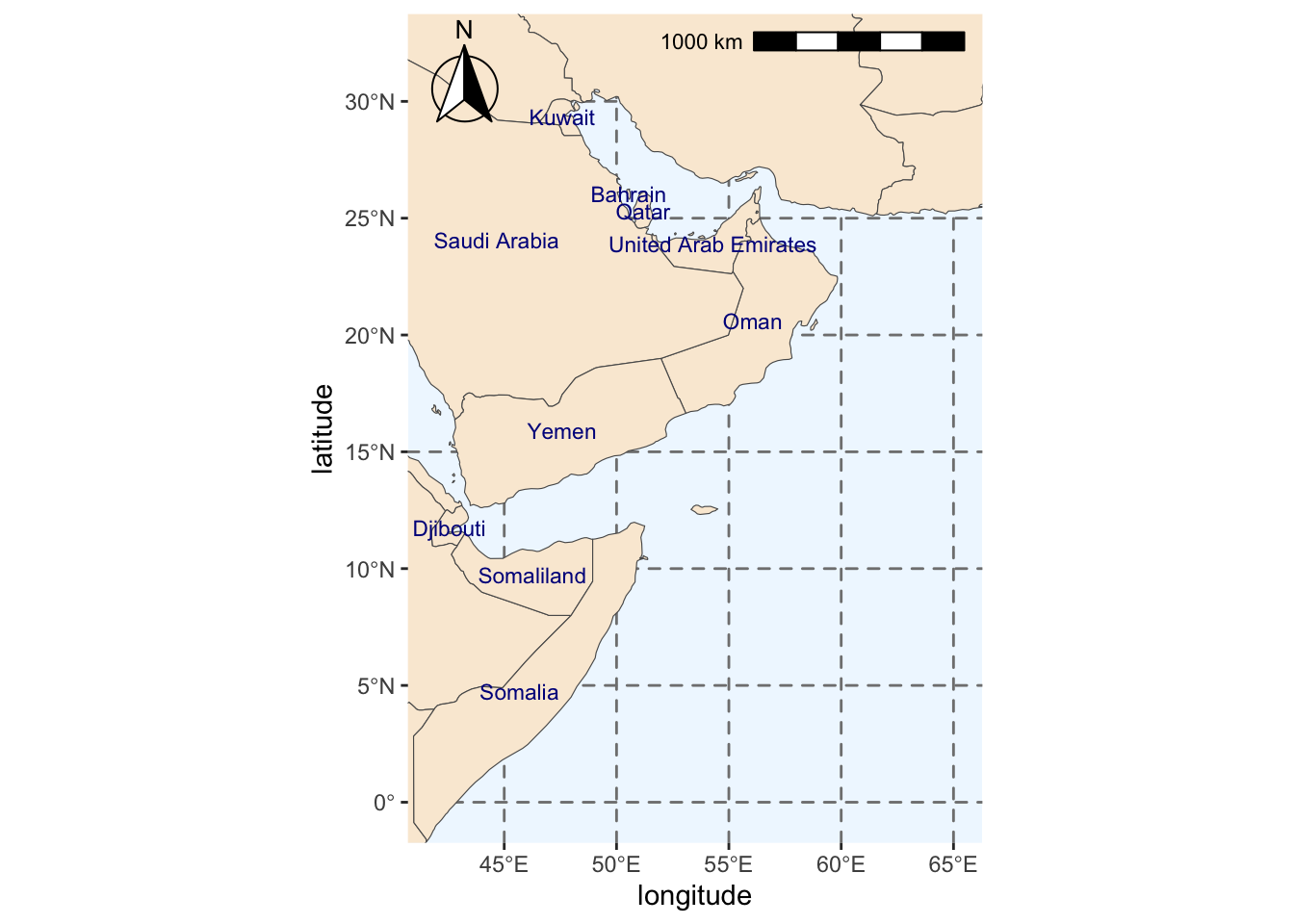

Loading in the save files

Later when we need the extent polygon, we use

#Loading bounding box for the area of interest
fil <- here::here("data", "region", "BoundingBox.shp")
extent_polygon <- read_sf(fil)

We often will need a sf bbox (bounding box object). To create that from the sf polygon object use

bbox <- sf::st_bbox(extent_polygon)

We load the maps as

fil <- here::here("data", "region", "region_map_label.rda")
load(fil)