library(ggplot2)
library(sdmpredictors)
library(DT)
library(sf)
Linking to GEOS 3.11.0, GDAL 3.5.3, PROJ 9.1.0; sf_use_s2() is TRUElibrary(raster)Loading required package: spWe are going to download environment data layers using sdmpredictors R package. We need to specify the directory where we will do this. We created the env directory in the data directory for this purpose.
Ultimately we need to get a data frame with the environmental data for the occurrence and absence lat/lon locations.
library(ggplot2)
library(sdmpredictors)
library(DT)
library(sf)Linking to GEOS 3.11.0, GDAL 3.5.3, PROJ 9.1.0; sf_use_s2() is TRUElibrary(raster)Loading required package: spSet the directory where we will save environmental data layers.
dir_env <- here::here("data", "env")
options(sdmpredictors_datadir = dir_env)We will use the sdmpredictors R package which has marine data layers.
# choose marine
env_datasets <- sdmpredictors::list_datasets(terrestrial = FALSE, marine = TRUE)The dataframe is large. We will use the DT package to make the table pretty in html.
env_layers <- sdmpredictors::list_layers(env_datasets$dataset_code)
DT::datatable(env_layers)See the Background discussion on how we decided on the environmental variables that we would use from the sdmpredictors R package.
layercodes <- c("BO_sstmean", "BO_bathymean", "BO22_ph", "BO2_dissoxmean_bdmean", "BO2_salinitymean_ss", "BO2_chlomean_ss", "BO21_nitratemean_ss")We want to set rasterstack equal true to get one file for our variables. This will save the files to data/env and we can load the files in later steps.
env <- sdmpredictors::load_layers(layercodes, rasterstack = TRUE)Load the bounding box.
#Loading bounding box for the area of interest
fil <- here::here("data", "region", "BoundingBox.shp")
extent_polygon <- read_sf(fil)
Make a plot of all the layers cropped to our bounding box.
io.rast <- raster::crop(env, raster::extent(extent_polygon))
plot(io.rast) 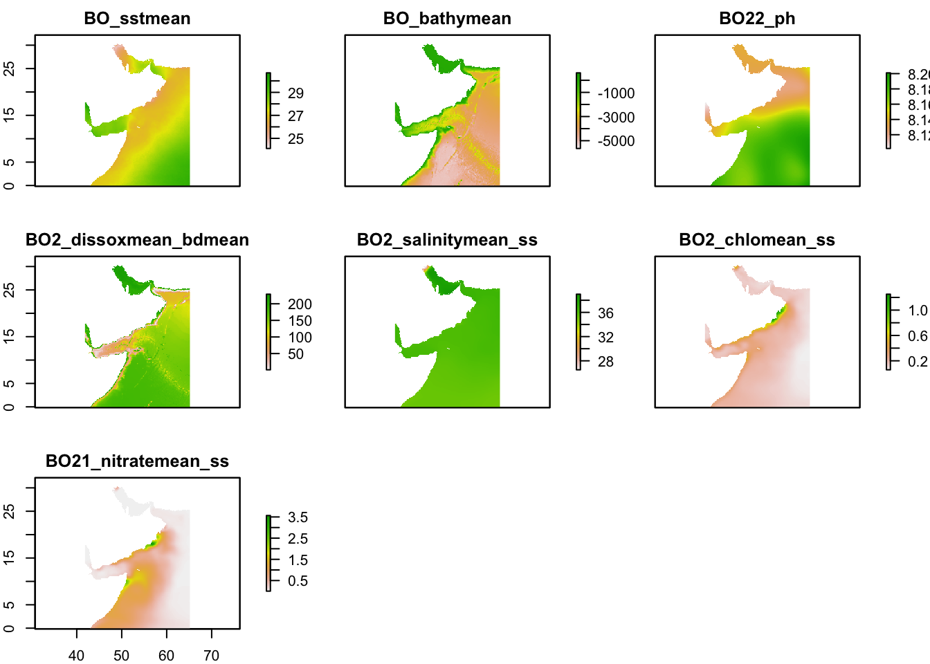
We will use the stars package to sample from our raster layers.
Load in our point data as data frames.
# presence data
fil <- here::here("data", "raw-bio", "io-sea-turtles-clean.csv")
df.occ <- read.csv(fil)

# absence data
fil <- here::here("data", "raw-bio", "pts_absence.csv")
df.abs <- read.csv(fil)
colnames(df.abs) <- c("lon", "lat")
Convert data frames to sf points objects. This is what stars needs.
df.abs <- na.omit(df.abs) # just in case
sf.abs <- sf::st_as_sf(df.abs, coords = c("lon", "lat"), crs = 4326)
sf.occ <- sf::st_as_sf(df.occ, coords = c("lon", "lat"), crs = 4326)
Convert the raster stack to a stars object.
env.stars <- stars::st_as_stars(env) # convert to stars object
env.stars <- terra::split(env.stars)
Get environment values for the absence points. Each row in sf.abs is a row in env.abs.
env.abs <- stars::st_extract(env.stars, sf::st_coordinates(sf.abs)) %>%
  dplyr::as_tibble() %>%
  na.omit()

head(env.abs)
# A tibble: 6 × 7
BO_sstmean BO_bathymean BO22_ph BO2_dissoxmean_bdmean BO2_salinitymean_ss
<dbl> <dbl> <dbl> <dbl> <dbl>
1 28.4 -2445 8.16 111. 36.2
2 26.9 -3142 8.12 119. 36.5
3 28.3 -4549 8.19 159. 36.0
4 27.1 -4970 8.17 180. 35.5
5 26.8 -3869 8.16 156. 36.0
6 28.0 -5095 8.17 183. 35.4
# ℹ 2 more variables: BO2_chlomean_ss <dbl>, BO21_nitratemean_ss <dbl>Get environment values for the occurence points. Each row in sf.occ is a row in env.occ.
env.occ <- stars::st_extract(env.stars, sf::st_coordinates(sf.occ)) %>%
  dplyr::as_tibble() %>%
  na.omit()

head(env.occ)
# A tibble: 6 × 7
BO_sstmean BO_bathymean BO22_ph BO2_dissoxmean_bdmean BO2_salinitymean_ss
<dbl> <dbl> <dbl> <dbl> <dbl>
1 28.6 -3158 8.18 154. 35.7
2 27.6 -8 8.13 198. 38.7
3 27.6 -4 8.13 198. 38.7
4 26.9 -2759 8.14 127. 36.1
5 26.9 -2067 8.14 98.6 36.0
6 27.6 -6 8.13 198. 38.7
# ℹ 2 more variables: BO2_chlomean_ss <dbl>, BO21_nitratemean_ss <dbl>Now make this into one data frame with a pa column for 1 is a occurrence row and 0 if an absence row.
pres <- c(rep(1, nrow(env.occ)), rep(0, nrow(env.abs)))
sdm_data <- data.frame(pa = pres, rbind(env.occ, env.abs))
head(sdm_data)
pa BO_sstmean BO_bathymean BO22_ph BO2_dissoxmean_bdmean BO2_salinitymean_ss
1 1 28.648 -3158 8.181 154.32448 35.73521
2 1 27.585 -8 8.133 197.65898 38.71139
3 1 27.553 -4 8.133 197.66029 38.65246
4 1 26.883 -2759 8.142 127.38091 36.10051
5 1 26.942 -2067 8.139 98.57215 36.04962
6 1 27.606 -6 8.133 197.74764 38.67334
BO2_chlomean_ss BO21_nitratemean_ss
1 0.107879 0.132562
2 0.141303 0.000003
3 0.141299 0.000002
4 0.293972 0.691326
5 0.517558 1.127677
6 0.141344 0.000002Save to a file. We will use for other models.
fil <- here::here("data", "raw-bio", "sdm_data.csv")
write.csv(sdm_data, row.names = FALSE, file=fil)